An
example of scattering
A common visualization problem is to draw curves in three dimensions.
We may want to draw streamlines for a fluid or gas, for example. It may
be difficult to interpret such plots, since it is hard to see if one
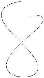
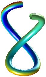
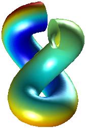
curve lies behind another. So, it is common to draw the curves as
ribbon or tubes instead. In the images below the leftmost curve is
drawn using the plot3-command
and in the other two the curve has been drawn as a tube. The leftmost
curve is almost impossible to interpret (at least if one has not seen
the tubes).
Using ribbons or tubes it is also possible to add information to a
curve. A ribbon can twist showing the rotation, curl, of the flow and a
tube can have a varying diameter, showing the divergence, for example
(see page 16-33 - 16-38 in the Matlab manual "3-D Visualization").
The Matlab commands streamline,
streamribbon and streamtube can draw streamlines
provided the input is presented in a mesh-form (as if produced by meshgrid). In the following
exercise we will not be able to use the existing commands, since a
curve is given as: (x(k), y(k), z(k)), k = 1, ..., n. This means that
you have to draw the ribbon yourself. Make a simple-minded
implementation. If you want a harder exercise, you can draw tubes
instead. Now to the visualization problem.
You have a group of stationary, point-charges situated around the
origin. We
shoot several particles (all with the same charge), at the group, and
your job is to draw the trajectories of the moving particles. This
problem is slightly harder than drawing streamlines, since the
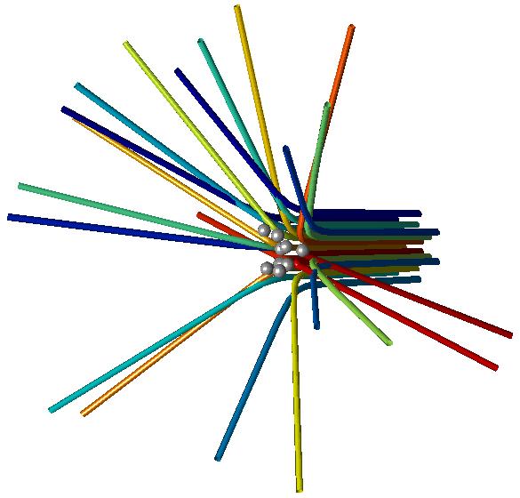
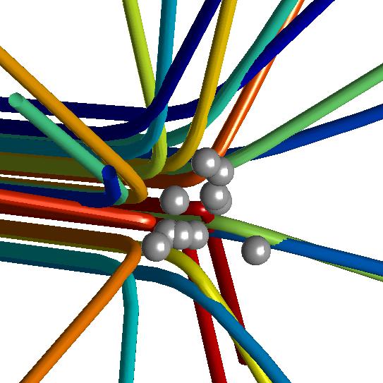
trajectories may intersect. This is what a typical image may look like
(I have drawn tubes using a tube-drawing command of my own
construction):
When looking at the image I would use the whole screen (the above image
is too small) and I would rotate it. In the following image I have
zoomed in:
The gray spheres are the stationary charged particles (they should be
points, but then we cannot see them clearly).
Now some mathematics. Let r(t)
= (x(t), y(t), z(t)), be the position of one moving particle. Assuming
Coulomb forces, no gravity etc., the differential equation for the
motion is given by (dropping (t) in r(t)):
r'' = c [ (r - p1) /
|| r -
p1 ||3 + (r - p2)
/
|| r - p2 ||3 + ... + (r -
pn) / || r - pn ||3
]
where p1, ..., pn are the
positions for the n fixed particles. c is a constant having to do with
the mass of the particle and the force between particles. || ||
denotes the ordinary two-norm (distance). Use ode45 two solve the system.
Test at least, the following configuration, defined by the code below:
global P c  % P and c are used in f
% P contains the coordinates for the fixed particles. One particle per column.
P = [
 -0.0466  0.0368  0.1156 -0.1553 -0.1079  0.1564  0.1155  0.1430  0.0826 0.1333
 -0.0516 -0.0825 -0.0364 -0.1542  0.0528 -0.1747  0.0316  0.0713  0.1680 0.0453
  0.1293  0.0281 -0.1349 -0.1852  0.1727 -0.0044 -0.1318 -0.1272 -0.1713 0.0056];

% The constant c is 0.001.
c = 0.001;

tspan = linspace(0, 15, 50);
phi_s = linspace(0, 2 * pi, 8);

% Find the trajectories for a few particles...
for R = [0.1 0.2 0.3]  % R is the radius, and not r
  for phi = phi_s(1:end-1)
    [t, y] = ode45(@f, tspan, [2 R*cos(phi) R*sin(phi) -0.3 0 0]');
%   more stuff ...
  end
end
If you do not know how to write f, you can find a version, ~thomas/VIS/Matlab/f.m, in the file system on the student machines.
When giving the initial conditions I have assumed that the positions
come first and then the velocities. So the initial position, for one
particle, is [2 R*cos(phi) R*sin(phi)] and
the initial velocity is [-0.3 0
0].
 So try to visualize the
trajectories using ribbons or tubes, where you have written your own
ribbon- or tube function.
So try to visualize the
trajectories using ribbons or tubes, where you have written your own
ribbon- or tube function.