Assignments
NOTE: THE DUE DATES FOR ASSIGNMENTS 2 TO 5 HAVE BEEN POSTPONED
There are five assignments in total. The first due date is rather late after the start to provide sufficient time to get acquainted with HPC. Do not underestimate the time it takes to solve an assignment. Notice that there are no lab sessions (and no lectures) during the weeks of April 10 to 21.
Please consider the submission instructions.
| Name | Due Date | Description |
|---|---|---|
| development environment | March 30, 2017 | Basic development tools. |
| optimization | April 06, 2017 | Performance measurement, diagnosis, and basic optimization. |
| threads | May 05, 2017 | POSIX threads. |
| openmp | May 12, 2017 | OpenMP, a compiler parallelization framework. |
| opencl | May 19, 2017 | Framework for heterogeneous computing environment (GPU, FMPG, etc.). |
| mpi | May 26, 2017 | Message passing interface for distributed computing. |
Development machine: Ozzy
Ozzy is a computer at the department of mathematics. You must have access to check and submit your assignments. I will give you an account after receiving your name, person number, and school. Do not forget to follow the requested format of your registration mail.
Ozzy does not allow for a graphical user interface, like all high performance computing environments. Use the terminal as explained in the first lectures.
Submission instructions
You are allowed and encouraged to work on and submit assignments in groups of three to four people.
After submitting, you will receive feedback on your assignment, and possibly a list of corrections that you have to make before passing on the assignment.
Do not diverge from the choice of programming language that is indicated for each of the exercises. If no choice is suggested, then it is mandatory to use C.
Report
In addition to the source code, you have to write a report in (pandoc compatible) markdown/commenmark that explains your solution, the program layout, and answers all questions posed in context of the task. You should discuss the program layout in the report first, and then consult with me to check that you have not missed any important point. Experience shows that otherwise extensive corrections are due.
Markdown
Markdown is a markup language which is geared towards easy typing and reading. If not familiar with it, you can find a summary of most important commands.
You can test whether you file compiles propertly with pandoc by running
pandoc report.markdownSubmission
Send your solutions to me by mail with subject “[HPCAssignment]” on the due day at the lastest.
Submission format
Your solution to assignments should be packaged as a tar.gz archive named by your lower case last names, separated by underscores.
Assignments may consist of several tasks. Each task should be implemented in a separate folder, and the main file for each task should follow the given naming convention. Include a make file that builds the program and cleans the build environment completely. Some assignments come with a test script, that unpacks, builds, and runs your programs, and also tests cleaning. If this is the case, make sure that your submission works with that script.
The report should be called “report.markdown” and be placed in the root folder of your solution archive. If you include any addition material (like pictures and graphs) in your report, then this should be contained in the folder material. I will compile the report using pandoc, so make sure to comply with its syntax.
Example
For example, in assignment 1, you have subtasks whose main files ought to be called “valgrind”, “profiling”, etc. A viable hand in by myself would thus be a file “raum.tar.gz” which contains the file “report.markdown” and folders named “material”, “valgrind”, “profiling”, etc. The folder material contains an image “profile_graph.png”, which is linked to from the report. The valgrind folder contains a “main.c” and several other C-files “addition.c”, “sin.c”, etc. Beyond that it contains a makefile that builds the program main when invoked.
Assignment 0: Development Environment
→ Back to the overview of assignments
The goal of this pre-assignment is to practice the basic use of the terminal environment and make. Send me your report as instructed.
LAPack and PLASMA
LAPack implements advanced linear algebra. PLASMA is a parallized variant.
Installing
Install PLASMA locally into the folder HOME/plasma_local from a TMux session. For this find the PLASMA installer on the web and run it on Ozzy. In the report describe the steps that you followed and the decisions that you made.
Use BLAS and LAPack that are installed on Ozzy. As opposed to this, you may download tmg and the LAPack C interface. You do not have to care about the choice of an efficient BLAS implementation.
Testing
Run the PLASMA tests; Report about how.
Makefile
Discuss the makefile used to compile the PLASMA tests, and the files that it includes directly or indirectly (these are three additional files).
Assignment 1: Optimization
→ Back to the overview of assignments
The goal of the first assignment is to practice how to time and profile code, and to inspect some aspects that contribute to performance. This is an assortment of six separate tasks. Send me your code and the report as instructed.
Time
Write a C program sum that computes naively and outputs the sum of the first billion integers. The makefile should contain a target “time” that times the programm by running it sufficiently often for all possible optimization levels (-O0 -O1 -O2 -O3 -Os -Og). It should also include a target assembler that creates the assembler output for all possible optimization levels. Discuss the timing results in light of the assembler code.
Inlining
Implement a function
void
mul_cpx( double * a_re, double * a_im, double * b_re, double * b_im, double * c_re, double * c_im)
that computes the product of two complex numbers b and c, and stores it in a. Write it (with different names) once in the same as the main function and once in a separate file. Write a program, called inlining, that generates vectors a, b, and c of length 30,000, generates entries for b and c, and then multiplies their entries, saving them to a. Benchmark this.
Inline the code of for multiplication, by hand, in the loop over a, b, and c. Benchmark once more, and compare the result. Reason about the difference.
Locality
Write a C program, called locality, that
- creates a matrix of doubles of size 1000 x 1000,
- stores them in a matrix in row first order,
- computes the row and the column sums.
Use naive implementations of row and column sums:
void
row_sums(
  double * sums,
  const double ** matrix,
  size_t nrs,
  size_t ncs
)
{
  for ( size_t ix=0; ix < nrs; ++ix ) {
    double sum = 0;
    for ( size_t jx=0; jx < ncs; ++jx )
      sum += matrix[ix][jx];
    sums[ix] = sum;
  }
}

void
col_sums(
  double * sums,
  const double ** matrix,
  size_t nrs,
  size_t ncs
  )
{
  for ( size_t jx=0; jx < ncs; ++jx ) {
    double sum = 0;
    for ( size_t ix=0; ix < nrs; ++ix )
      sum += matrix[ix][jx];
    sums[jx] = sum;
  }
}
Time them according to the above scheme. Compare timings and reimplement the slower summation in a more effective way. In addition, compile your program with and without full optimization. Summarize your timing results in a short table.
Indirect addressing
Indirect addressing is frequently used for sparse matrix and vector operators. Write a C or C++ program that increments a vector y by a multiple of a vector x. Both vectors will have same length 1,000,000 and the index vector (as opposed to real world applications) has also that length.
Implement, as a program called indirect_addressing, code
n = 1000000; m = 1000;
for (kx=0; kx < n; ++kx) {
  jx = p[kx];
  y[jx] += a * x[jx];
}
and benchmark it with some vectors x and y, and scalar a, and with p generated by either
ix = 0;
for (jx=0; jx < m; ++jx)
  for (kx=0; kx < m; ++kx)
    p[jx + m*kx] = ix++;
or
for (ix=0; ix < n; ++ix)
  p[ix] = ix;
Also implement and benchmark the same operation without indirect addressing, i.e. by accessing x and y directly.
Use once full and once no optimization in all cases. Compare the timings, and explain the difference.
Valgrind
Implement a function that allocates an array of 1000 ints without freeing them. Call it in a program called leak before computing naively and printing the sum of first one billion integers. Write a makefile target check that runs the program with valgrind memcheck. Discuss the valgrind output in your report.
Profiling
Using the tools gprof and gcov to inspect your implementation row and column sums of a matrix. Compare with bash timings. Also identify those parts that are most frequently run.
Assignment 2: Threads
→ Back to the overview of assignments
NOTE: THE DUE DATES FOR ASSIGNMENTS 2 TO 5 HAVE BEEN POSTPONED
We will use Newton’s method to practice programming with POSIX threads. Give a function f, say f(x) = x^3 - 1, Newton’s method iteratively strives to find a root of f. Starting with a value x_0, one sets x_{k+1} = x_k - f(x_k) / f’(x_k). Convergence of this is unclear, and even if it does converge, it is unclear what root of f is approached.
Here is an example run of Newton’s method for three different (complex) values of x_0.
| real value | complex value | complex conjucate of previous one | |
|---|---|---|---|
| x_0 | 4.00000000000000 | -3.00000000000000 + 1.00000000000000i | -3.00000000000000 - 1.00000000000000i |
| x_1 | 2.68750000000000 | -1.97333333333333 + 0.686666666666667i | -1.97333333333333 - 0.686666666666667i |
| x_2 | 1.83781773931855 | -1.25569408339907 + 0.505177535283118i | -1.25569408339907 - 0.505177535283118i |
| x_3 | 1.32390198935733 | -0.705870398114610 + 0.462793270024375i | -0.705870398114610 - 0.462793270024375i |
| x_4 | 1.07278230395299 | -0.284016534261040 + 0.737606186335893i | -0.284016534261040 - 0.737606186335893i |
| x_5 | 1.00482620484690 | -0.585120941952759 + 0.849582155034797i | -0.585120941952759 - 0.849582155034797i |
| x_6 | 1.00002314326798 | -0.501764864834321 + 0.859038339628915i | -0.501764864834321 - 0.859038339628915i |
| x_7 | 1.00000000053559 | -0.499955299939949 + 0.866052541624328i | -0.499955299939949 - 0.866052541624328i |
One can experimentally find which points on the complex plane converge to which root. Below there are two pictures: In the left one every pixel is colored in such a way that its color corresponds to the root which it converges to. In the right hand side, every pixel is color in such a way that its color corresponds to the number of iterations which are necessary to get close to a root of f. Note that this computation can be carried out for each pixel in parallel. There is no interdependence among the iterations.


Implementation
Implement in C using POSIX threads a program called newton that computes similar pictures for a given functions f(x) = x^d - 1 for complex numbers with real and imaginary part between -2 and +2. The program should write the results as ppm files to the current working directory. The files should be named newton_attractors_xd.ppm and newton_convergence_xd.ppm where d is replaced by the exponent of x that is used.
If x_i is closer than 10^-3 to one of the roots of f(x), then abort the iteration. Newton iteration does not converge for all points. To accomodate this, abort iteration if x_i is closer than 10^-3 to the origin, or if the absolute value of its real or imaginary part is bigger than 10^10. In the pictures treat these cases as if it was an additional zero of f(x) to which these iterations converge.
Your program should accept command line arguments
./newton -t5 -l1000 7The last argument is d, the exponent of x in x^d - 1. The argument to -l gives the number of rows and columns for the output picture. The argument to -t gives the number of threads used to compute the pictures. For example, the above command computes images of size 1000x1000 for the polynomial x^7 - 1. It uses 5 threads for the Newton iteration. You find an example program at
/home/hpc01/a2_grading/example/newton -t2 -l1000 5Besides the threads to compute the iteration you may use one main thread for convenience and one thread that writes to disc. Neither of them may compute the newton iteration. The implementation should compute the pictures row by row.
If you use optimization techniques that require different parameters for different sets of arguments -t and -l then you are allowed to choose suitable parameters before launching threads. It is acceptable to determine the optimal values for the performance goals below.
Test script
You can check your submission with the script
/home/hpc01/a2_grading/check_submission.pyPerformance goals
The program will be tested with the following parameters. It must be at least as fast as given in the corresponding tables.
Single threaded, 1000 lines, varying polynomial x^d - 1
| Degree of polynomial | 1 | 2 | 5 | 7 | |
| Maximal runtime in seconds | 0.246 | 0.292 | 3.876 | 5.600 |
Multithreaded, 1000 lines, x^5 - 1
| Number of threads | 1 | 2 | 3 | 4 | |
| Maximal runtime in seconds | 3.876 | 2.058 | 1.488 | 1.176 |
Ten threads, varying number of lines, x^7 - 1
| Number of lines | 1000 | 50000 |
| Maximal runtime in seconds | 0.798 | 1055 |
PPM files
PPM (Portable PixMap) files are an ASCII based image format. You can write and read them as a text file. Wikipedia contains a description with examples. In this assignment the header must look like
P3
L L
M
where L is the number of rows and columns and M is the maximal color value used in the body of the file.
Assignment 3: OpenMP
→ Back to the overview of assignments
NOTE: The performance goals have been corrected
In this assignment, we count in parallel distances between points in 3-dimensional space. On possibility to think of this, is as cells whose coordinates were obtained by diagnostics, and which require further processing.
Distances are symmetric, i.e. distance between two cells c_1 and c_2 and the distance in reverse direction c_2 to c_1 should be counted once.
Implementation
Implement a program in C, called cell_distances, that uses OpenMP and that:
- Reads coordinates of cells from a text file “cells” in the current working directory. You may assume that coordinates are between -10 and 10.
- Computes the distances between cells counting how often each distance rounded to 2 digits occurs.
- Outputs to stdout a sorted list of distances with associated frequencies (including 0 fequencies at your will).
Your program should accept command line arguments
./cell_distances -t5The argument to -t give the number of OpenMP threads that you may use. You may only use OpenMP parallelism. You find an example program at
/home/hpc01/a3_grading/example/cell_distances -t10Your programm at no time may consume more than 1 gigabyte of memory.
Example
The list of positions is given as a file of the form
+01.330 -09.035 +03.489
-03.718 +02.517 -05.995
+09.568 -03.464 +02.645
-09.620 +09.279 +08.828
+07.630 -02.290 +00.679
+04.113 -03.399 +05.299
-00.994 +07.313 -06.523
+03.376 -03.614 -06.657
+01.304 +09.381 -01.559
-04.238 -07.514 +08.942
A valid output, ignoring rounding errors, which will be tolerated in the submission tests, is
03.00 1
05.54 1
05.85 1
05.91 1
06.07 1
06.54 1
07.94 1
08.58 1
09.40 1
09.59 1
09.65 1
09.98 1
10.00 1
11.18 1
11.68 1
11.77 1
11.98 1
13.46 1
14.02 1
14.11 1
14.77 1
14.78 1
14.96 1
15.07 1
15.38 1
15.71 1
15.78 1
15.84 1
16.75 1
16.94 1
17.33 1
17.63 1
17.66 1
17.72 1
17.79 1
18.00 1
19.02 1
19.10 1
19.31 1
20.65 1
21.67 1
22.00 1
22.31 1
23.85 1
23.98 1
Test script
You can check your submission with the script
/home/hpc01/a3_grading/check_submission.pyNotice that the test script
- checks your output for correctness,
- redirects stdout to a file, so that additional runtime costs for writing to disc can apply.
Performance goals
| Number of points | 1e4 | 1e5 | 1e5 | 1e5 |
| Number of threads | 1 | 5 | 10 | 20 |
| Maximal runtime in seconds | 0.54 | 13.4 | 6.62 | 3.98 |
Assignment 4: OpenCL
→ Back to the overview of assignments
A simple model for heat diffiusion in 2-dimensional space, splits it up into n_x times n_x small boxes. In each time step, the temperature h(i,j) of a box with coodinates i and j is updated as
h(i,j) + c * ( (h(i-1,j) + h(i+1,j) + h(i,j-1) + h(i,j+1))/4 - h(i,j) )
where c is a diffision constant. We consider the case of bounded region of box shape whose boundary has constant temperature 0.
Implementation
Implement in C using the GPU via OpenCL a program heat_diffusion that
- Initializes an array of given size to 0 except for the middle point whose initial value is determined by a parameter -i.
- Executes a given number of steps of heat diffusion with given diffusion constant, and
- Outputs the average a of temperatures.
- Outputs the average absolute difference of each temperature to the average of all temperatures.
Your program should accept command line arguments
./heat_diffusion 1000 100 -i1e10 -d0.02 -n20to compute with boxes of size width 1000, height 100, initial central value 1e10, diffusion constant 0.02, and 20 iterations. You may only use OpenCL parallelism. You find an example program at
/home/hpc01/a4_grading/example/heat_diffusion 1000 100 -i1e10 -d0.02 -n20OpenCL on Ozzy
To build an OpenCL program on Ozzy, you have to use the respective CUDA bindings. To build your program add the following flags
-I/usr/local/cuda-7.5/targets/x86_64-linux/include -L/usr/local/cuda-7.5/targets/x86_64-linux/lib -lOpenCLWhile unlikly, the path to CUDA could change during the course. In doubt, contact me about this.
Example
As an example, we consider the case of 3 times 3 boxes with diffusion constant 1/30. Their initial heat values written in a table are
| 0 | 0 | 0 |
| 0 | 1,000,000 | 0 |
| 0 | 0 | 0 |
Then the next two iterations are
| 0 | 8333 | 0 |
| 8333 | 9667e2 | 8333 |
| 0 | 8333 | 0 |
and
| 138.9 | 1611e1 | 138.9 |
| 1611e1 | 9347e2 | 1611e1 |
| 138.9 | 1611e1 | 138.9 |
In particular, the average temperature is 111080 (as opposed to the original average 111111).
The absolute difference of each temperature and the average is
| 1109e2 | 9497e1 | 1109e2 |
| 9497e1 | 8236e2 | 9497e1 |
| 1109e2 | 9497e1 | 1109e2 |
with average is 183031.55. After five further iterations this will decrease to 151816.97.
Performance goals
Note that the NVidea driver on Ozzy consumes significant time to start up (this will be accounted for by 5.7 seconds). This time has been considered in the goals below.
| Width * Height | 100 * 100 | 10000 * 10000 | 100000 * 100 |
| Initial value | 1e20 | 1e10 | 1e10 |
| Diffusion constant | 0.01 | 0.02 | 0.6 |
| Number of iterations | 100000 | 1000 | 200 |
| Time in seconds | 7.26 | 100 | 7.0 |
Assignment 5: MPI
→ Back to the overview of assignments
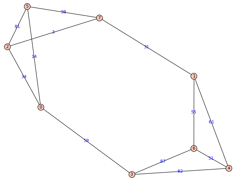
Dijkstra’s algorithms finds shortest paths in graphs with directed, weighted edges. In the following example of a symmetric (i.e. undirected) graph is, a shortest path from node 2 to node 4 would go via node 1 and node 7.
One can implement Dijkstra’s algorithm via MPI: Every worker gets assigned a fixed set of nodes. In every iteration, each worker updates its unvisited neighbore to the current node. The minimal tentative distance among all nonvisited nodes can also be determined by a distributed computation.
Implementation
Implement the described algorithm as a program called dijkstra in C using MPI. The program should output the length of a shortest path in the graph from a given source to a given destination.
mpirun -n 1 dijkstra 2 4 example_graphYou can call an example program via
ln -sf /home/hpc01/a5_grading/test_data/graph_de1_ne3_we2 graph && mpirun -n 1 /home/hpc01/a5_grading/example/dijkstra 1 17 graphGraph input file
Your program should read the graph from a given file with lines of the form
i1 i2 wwhere i1 and i2 are indices of vertices connected by an edge of weight w. The first two columns are the lable of a vertices, a positive integer, and the third one is a weight, an integer greater than 0. The above graph would, for example, yield
0 2 34
0 3 59
0 5 14
1 4 61
1 6 55
1 7 31
2 0 34
2 5 81
2 7 3
3 0 59
3 4 82
3 6 87
4 1 61
4 3 82
4 6 51
5 0 14
5 2 81
5 7 98
6 1 55
6 3 87
6 4 51
7 1 31
7 2 3
7 5 98
Note that the this graph has undirected edges, so that the table of weights is symmetric.
Examples of Graphs
You can find a list of test graphs at
/home/hpc01/a5_grading/test_dataThere is also a python script, that you can use to generate test cases for you convenience.
Performance goals
For the files that can be found at
/home/hpc01/a5_grading/test_data| Degree | 10 | 100 | 100 | 100 | 1000 |
| Number of vertices | 1000 | 10000 | 10000 | 100000 | 100000 |
| Maximal weight | 100 | 100 | 100 | 100 | 1000 |
| File name | graph_de1_ne3_we2 | graph_de2_ne4_we2 | graph_de2_ne4_we2 | graph_de2_ne5_we2 | graph_de3_ne5_we3 |
| Number of nodes | 1 | 1 | 4 | 10 | 20 |
| Start point | 9 | 17 | 17 | 107 | 4 |
| End point | 82 | 40 | 18 | 0 | 5 |
| Time in seconds | 0.26 | 9.92 | 2.64 | 97 | 472 |