Assignments
There are six assignments in total, four of which are mandatory. Solutions of Assignments 4 and 5 count towards you examination. The first due date is rather late after the start to provide sufficient time to get acquainted with HPC. Do not underestimate the time it takes to solve an assignment.
Please consider the submission instructions.
| Name | Due Date | Description |
|---|---|---|
| development environment | Mo, September 17 | Basic development tools. |
| optimization | Mo, October 1 | Performance measurement, diagnosis, and basic optimization. |
| threads | Mo, October 15 | POSIX threads. |
| openmp | Fr, October 26 | OpenMP, a compiler parallelization framework. |
| opencl (optional) | Fr, October 26 | Framework for heterogeneous computing environment (GPU, FPGA, etc.). |
| mpi (optional) | Tu, October 30 | Message passing interface for distributed computing. |
All assignment texts are by Martin Raum, CC BY-SA 4.0.
Submission instructions
There are two types of assessments. I will assess directly your solutions to Assignments 2 and beyond. For them your program’s performance is the key objective. You handle Assignments 0 and 1 yourself as peer assessments. The focus of peer assessed assignments is to enforce learning of basic techniques that you will need for the remaining assignments.
Peer assessment
For peer assessment, first solve the assignments independently. Then get together in groups of three to check and possibly improve your solutions in group work. You can then come forward to me or Johannes during the computer lab sessions. After possibly asking some questions for cross-check, we will register your passing the assignment.
Performance assessment
Send your solutions to all assignments that I assess to me by mail with subject “[HPCAssignment]” on the due day at the lastest. Delayed submissions will not be accepted. After submission you will receive feedback on your assignment and possibly a list of corrections that you have to make before you pass the assignment. Make sure before submitting that your solutions passes the check scripts that I provide.
Submission groups
For Assignments 2 and beyond you are allowed and encouraged to work on and submit assignments in groups of two or three students. You have to sign up for a group tag that I will assign for the purpose of tracking your submissions. For example, hpcgp001 would be such a tag. You send email to me with subject “[HPCGroup]” with a list of all usernames on gantenbein that be part of your group. I will answer with a group tag. For instance, if you have accounts hpcuser021, hpcuser043, and hpcuser056 that wish to work together as a group, then send me a mail
hpcuser021, hpcuser043, hpcuser056
and I would, for example, reply by
hpcgp000
Implementations and source code
Programming language
Do not diverge from the choice of programming language that is indicated for each of the exercises. If no choice is suggested, then it is mandatory to use C.
Makefile build
You have to include a makefile, whose standard target builds all required exectuables. For example, if you have to provide exectuables main1 and main2, then the following must work
make
./main1
./main2
Makefile clean
The makefile must also provide a clean target that shall remove all files resulting from compilation, but no more. For example, if you provide two files, main.c and makefile, and running the exectuable main yields another file called outputfile, then
make
./main
make clean
should preserve main.c, makefile, and outputfile, but delete main.o (if created) and main.
Build system
Your code must compile and run on gantenbein.
Report
In addition to the source code for your solution, you have to write a report in (kramdoc compatible) markdown that explains your solution, with focus on the program layout and performance characteristics. You shall also answers all questions posed in context of the assignment, if there is any.
Markdown
Markdown is a markup language which is geared towards easy typing and reading. If not familiar with it, you can find a summary of most important commands.
You can test whether you file compiles propertly with kramdown by running
kramdown report.md -o html > report.html
Submission archive
Your solution to assignments should be packaged as a tar.gz-archive named by your group tag in lower case letters. For example, if your tag is hpcgp001, then your submission should contain one tar.gz-archive hpcgp001.tar.gz.
Report
The root directory of the submission tar.gz-archive should contain the report as file called report.md. If you include any addition material (like pictures and graphs) in your report, then this should be contained in the folder reportextra. For example, if hpcgp001 is your group tag, then
tar xf hpcgp001.tar.gz
kramdown report.md -o html > report.html
should create an html-file from your report.
Example
The following example assignment is unrelated to any of the actual assigments. The purpose of this example is to illustrate concretely what aspects you should treat in your report.
Tasks description
Implement a program called randomtyping that
- prints to the command line a random nonnegative number with at most three digits,
- waits for the user to enter a nonnegative number,
- checks whether these numbers match; if they do not the program exits.
You can freely assume that the user input will yield machine size integers.
Submission archive
An implementation of this can be found in this following tar-archive.
Report
The report, also contained in the above submission archive, addresses the program layout first and then performance. For this very small program, the program discussion is comparatively detailed, essentially discussion every single line. In your actual submission it suffices to discuss blocks of code that serve a given purpose (semantic blocks). The performance evuluation is meant humourous, but reveals the essential features of an actual discussion: Identify what you believe (or know) are the limiting factors to performance and elaborate on alternative implementations. A comparison of benchmarks as in the example is not required, but can be of great value also to your developing the program.
Development machine: Gantenbein
→ Back to the overview of assignments
Gantenbein is a computer at the department of mathematics. You must have access to check and submit your assignments. I will give you an account after you have registed in PingPong. Come and see me during the first lab session.
If you, for instance, have the user name hpcuser023, you log into gantenbein via
ssh hpcuser023@gantenbein.math.chalmers.se
After that you have a usual terminal to work in. Gantenbein does not allow for a graphical user interface, like all high performance computing environments. Use the terminal as explained in the first lectures.
Editing files on gantenbein
There are two standard text editors installed on gantenbein: NeoVim and Emacs. For beginners I very much recommend to use Emacs. You can open a file for editing by
emacs FILENAME
Navigation within a file works, for example, with key arrows. To write a file to disc press CTRL-x CTRL-s. To close a file press CTRL-x CTRL-c.
Transfering files to and from gantenbein
Should you want to edit files on a different system, you will need means to transfer them to and from gantenbein. I will not give you support on this, since the officially recommended way is to work on gantenbein directly.
Here, though, is some information for your convenience: The most confortable way is to use sshfs, which is available to you if you use your own Linux, Mac, or Windows computer. It connects a folder on gantenbein with a folder on your computer in a persistent way. To transfer individual folders or files, you can use the command scp on Linux and Mac. The user manual can be retrieved by the man command, as explained in the lectures.
If you decide to take files on your own computer, but do not have a suitable code editor, Atom is a popular one that runs on Linux, Mac, and Windows. Yet again, though, I will not provide support for running this on your system.
Assignment 0: Development Environment and basic programming
→ Back to the overview of assignments
The goal of this pre-assignment is to practice the basic use of the terminal environment and make. This is subject to peer-assessment.
Loging in and setting up a terminal environment
Make sure to revisit from the lectures’s slides how to:
- Log into gantenbein via ssh.
- Start and use the terminal multiplexer tmux.
- Build a project via make.
Flint and Arb
Arb is a library for arbitrary precision ball arithmetic. It builds up on Flint, a library for fast number theoretic comuputation. The next goal is to provide local installations of both on gantenbein. You will need to install Flint first and then Arb.
Acquiring the code
Many programs that one uses in an HPC environment are not provided by the system. You have to find them yourself, often on the web. Make sure to:
- Find both Flint 2.5 and Arb 2.14 on the web.
- Download the source code to your home directory or a suitable subfolder.
Using Git
The following is optional for those, who wish to train the use of git.
- Find the git repositories of Flint and Arb.
- Clone them to build the very latest versions instead of versions 2.5 and 2.14, respectively.
- Discuss what is the advantage and disadvantage of using such not yet released code?
- When inspecting the git history of Flint, how do such general arguments apply to the case at hand?
Installing Flint
To build and install Flint, find the readme file in the Flint source folder and follow the instructions. When configuring the build make sure that:
- Flint is built using the native processor architecture (GCC target architecture) of gantenbein.
- Flint is installed into HOME/local_flint, where HOME is your home directory.
- Flint is built using the system-wide installation of MPIR and MPFR. Notice that the install documentation of Flint is inaccurate when it comes to detecting both.
Installing Arb
Adjust the steps that you follows for installing Flint to Arb. In particular, you will have to find a way how to inform the Arb configuration about where you have installed Flint. Make sure that:
- Arb is built using the native processor architecture (GCC target architecture) of gantenbein.
- Arb is installed into HOME/local_arb, where HOME is your home directory.
Testing your installation
Flint comes with a small set of tests. Find out how to build and run them.
- Verify that your installion of Flint runs its tests correctly.
Arb comes with a small set of examples.
- Copy the example poly_roots.c into a separate folder.
- Write a makefile to build it.
- Verify the functioning of the resulting program.
Basic C programming
The basic layout of C programs is similar to other programming languages, Java for example. A reference can be found at cppreference.com. It is important to be familiar with the syntax of if, for, and while statements, which are merely a syntactic variation of what can be found in other programming languages. The next goal is to get familiar with the basic pattern of stack allocation, heap allocation, and file access.
Stack allocation
Allocation describes the reserving of memory for a program. Stack allocation is the fastest variant. While the C standard makes no assumption on what memory is allocated on the stack, it is reasonable to assume that arrays of static size are allocated on the stack.
Write a program employing the following allocation pattern
#define SIZE 10

int as[SIZE];
for ( size_t ix = 0; ix < SIZE; ++ix )
  as[ix] = 0;

printf("%d\n", as[0]);
Make sure that you place the declaration of the array as the main function (as opposed to global scope).
Compile and run the program with optimization level 1 on gcc. Then increase the size of the arrary, recompile and run, until the program fails with a segmentation fault. Explain this behavior assuming that that allocation was performed on the stack.
Heap allocation
Heap allocation is the alternative to stack allocation. It is generally slower, but more flexible. In particular, it has less restrictions on the size of allocated memory.
Write a program with the following allocation pattern
#define SIZE 10

int * as = (int*) malloc(sizeof(int) * SIZE);
for ( size_t ix = 0; ix < SIZE; ++ix )
  as[ix] = 0;

printf("%d\n", as[0]);

free(as);
Compile and run as above, and verify that the program does not fail for sizes that triggered a segmentation fault before.
Reducing memory fragmentation
When allocating memory on the heap, there is no guarantee about where it is positioned. A common strategy to avoid this is to allocate memory in large blocks (contiguous memory). Implement a program based on the next two code snippets. Explain the meaning of all variables, and exhibit the possible layout of allocated memory in both cases.
Not avoiding memory fragmentation:
#define SIZE 10

int ** as = (int**) malloc(sizeof(int*) * SIZE);
for ( size_t ix = 0; ix < SIZE; ++ix )
  as[ix] = (int*) malloc(sizeof(int) * SIZE);

for ( size_t ix = 0; ix < SIZE; ++ix )
  for ( size_t jx = 0; jx < SIZE; ++jx )
    as[ix][jx] = 0;

printf("%d\n", as[0][0]);

for ( size_t ix = 0; ix < SIZE; ++ix )
    free(as[ix]);
free(as);
Avoiding memory fragmentation:
#define SIZE 10

int * asentries = (int*) malloc(sizeof(int) * SIZE*SIZE);
int ** as = (int**) malloc(sizeof(int*) * SIZE);
for ( size_t ix = 0, jx = 0; ix < SIZE; ++ix, jx+=SIZE )
  as[ix] = asentries + jx;

for ( size_t ix = 0; ix < SIZE; ++ix )
  for ( size_t jx = 0; jx < SIZE; ++jx )
    as[ix][jx] = 0;

printf("%d\n", as[0][0]);

free(as);
free(asentries);
Writing to files
The C file model is based on FILE pointers, which have to be acquired and released. Check on the web the syntax and meaning of the following functions:
- fopen
- fclose
- fprintf
- fscanf
- fwrite
- fread
- fflush
Implement a program that
- opens a file for writing,
- writes a square matrix of size 10 with int entries (any at your will) to that file,
- closes and reopens the file for reading,
- reads the matrix from the file,
- and compares entrywise with the original one.
How does your choice of memory allocation (contiguous vs. noncontiguous) impact the possibilties to write the matrix?
Parsing command line arguments
Programs can be called with command line arguments. For example, a program printargs might be called as
./printargs -a2 -b4
These arguments are passed to the main function
int
main(
    int argc,
    char *argv[]
    )
as an array of null-terminated strings argv (argument vector), the number of which is argc (argument count). In the above example the argument count is 3 and the argument vector accordingly contains 3 strings “./printargs”, “-a2”, and “-b4”.
Make sure that you are familiar with the concept of null-terminated strings and stdout and check on the web the syntax and meaning of the following functions and expressions:
- == ‘a’ (as opposed to == “a”)
- strcmp
- strtol
- printf
Implement a program that
- accepts two arguments -aA and -bB for integers A and B in arbitrary order, i.e. -aA -bB and -bB -aA are both legitimate arguments when calling your program,
- converts A and B to integers, and
- writes to stdout the line “A is (INSERT A) and B is (INSERT B)”.
For example calling
printargs -a2 -b4
or
printargs -b4 -a2
should output
A is 2 and B is 4
As a final remark observe that standard programs would equally accept “-a2” and “-a 2”. When using standard solutions like POSIX getopt, this is automatically taken care of.
Learning summary
This assignment is a preparation towards your working on Assignments 2 through 5. In particular, you will need the following to facilitate your course studies:
- From the first part, it is very helpful to keep in mind the use of makefiles. They save you a lot of time when recompiling, and make the use of compiler flags more transparent. When coding and then rerunning your program, you might want to use commands like
make && ./program_with_parameters -
From the second and third part, it is helpful to remember that stack memory can be much faster, but its size is limited. Once you can argue that an array fits on the stack, it is preferable to allocate it there.
-
From the fourth part, it is helpful to remember both memory allocation patterns. Contiguous memory allocation is typically faster, but it is also less flexible. That is, using contiguous memory allocation you are forced to allocated the required memory at once. As for non-contiguous memory allocation you can allocate and free each row whenever it is optimal in your code.
-
From the fifth part, it is helpful to record that fprintf is potentially much slower than fwrite. In particular, when writing the same string repeatedly in a program, it can be helpful to prepare a string in memory (i.e. an array of char) via, for example, sprintf and then write it to file employing fwrite.
- From the sixth part, it is helpful to remember the programming pattern. Most programs need to parse command line arguments. You can reuse the code that you have written in other assignments.
Assignment 1: Optimization
→ Back to the overview of assignments
The goal of the first assignment is to practice how to time and profile code, and to inspect some aspects that contribute to performance. This is an assortment of various, independent tasks that are subject to peer assessment. It is allowed and suggested to complete each task, and then consult with your peer assessment group for feedback before starting the next task. Only after completing all tasks, however, you need to register your passing with me or Johannes.
Time
In this task you familiarize yourself with a naive approach to timing and benchmarking. Familiarize yourself with
- the datatype timespec and
- the function timespec_get.
Implement a program that
- in a loop repeats,
- the naive computation of the sum of the first billion integers,
- writing the result to stdout,
- takes the time before and after the loop,
- computes the runtime of a single loop iteration from the difference of start and stop time.
Compile and run the program with all possible optimization levels (-O0 -O1 -O2 -O3 -Os -Og). Also generate assembler code for each of the optimization levels. Discuss the timing results in light of that assembler code.
Inlining
In this task you will see the effect of automatic inlining. You have to compile programs with optimization level 2 (i.e. compiler flag -O2) in order to produce theeffect.
Implement a function with signature
void
mul_cpx( double * a_re, double * a_im, double * b_re, double * b_im, double * c_re, double * c_im)
that computes the product of two complex numbers b and c, and stores it in a. The suffices re and im stand for the real and imaginary part of a,b,c respectively.
- Provide two identical implementations of this function, with two different names mul_cpx_mainfile and mul_cpx_separatefile, once in the same file as the main function and once in a separate c-file. Recall to this end that you have to provide and include a corresponding header file in the second case.
- Write a program, called mainfile, that
- generates vectors as, bs, and cs of length 30,000,
- generates entries for bs and cs (any kind of entries will do), and then
- multiplies the entries of bs and cs using mul_cpx_mainfile, saving results to as.
- Write a program, called separatefile, that
- generates vectors as, bs, and cs of length 30,000,
- generates entries for bs and cs (any kind of entries will do), and then
- multiplies the entries of bs and cs using mul_cpx_separatefile, saving results to as.
- Write a program, called inlined, that
- generates vectors as, bs, and cs of length 30,000,
- generates entries for bs and cs (any kind of entries will do), and then
- multiplies the entries of bs and cs saving results to as by inserting the implementation of mul_cpx into the main-function by hand.
- Benchmark each of the three variants and reason about the difference.
- Use the tool nm to examine the first two executables for symbols that correspond to mul_cpx_mainfile and mul_cpx_separatefile. Do you find them in both cases?
Locality
Write a C program, called locality, that
- creates a matrix of doubles of size 1000 x 1000,
- stores them in a matrix in row major order,
- computes the row and the column sums.
Use the following naive implementations of row and column sums:
void
row_sums(
  double * sums,
  const double ** matrix,
  size_t nrs,
  size_t ncs
)
{
  for ( size_t ix=0; ix < nrs; ++ix ) {
    double sum = 0;
    for ( size_t jx=0; jx < ncs; ++jx )
      sum += matrix[ix][jx];
    sums[ix] = sum;
  }
}

void
col_sums(
  double * sums,
  const double ** matrix,
  size_t nrs,
  size_t ncs
  )
{
  for ( size_t jx=0; jx < ncs; ++jx ) {
    double sum = 0;
    for ( size_t ix=0; ix < nrs; ++ix )
      sum += matrix[ix][jx];
    sums[jx] = sum;
  }
}
With an eye to memory access patterns
- benchmark both variants and compare timings, then
- reimplement the slower summation in a more effective way.
To conclude
- compile your program with optimization level 0 and 2, and
- summarize and explain your timing results.
Indirect addressing
In this task you get familiar with the impact of indirect addressing. It is frequently used for sparse matrix and vector operators.
Write a program that
- increments a vector y by a multiple of a vector x, both of which have length 1,000,000.
- the index vector (as opposed to real world applications) has also that same length.
Concretely, implement, as a program base on the following code:
n = 1000000; m = 1000;
for (kx=0; kx < n; ++kx) {
  jx = p[kx];
  y[jx] += a * x[jx];
}
Benchmark two variants of the program for some fix vectors x and y (any kind of entries will do), and some nonzero scalar a, where p is generated by either
ix = 0;
for (jx=0; jx < m; ++jx)
  for (kx=0; kx < m; ++kx)
    p[jx + m*kx] = ix++;
or
for (ix=0; ix < n; ++ix)
  p[ix] = ix;
Provide and benchmark an alternative implementation that accesses x and y directly, avoiding indirect addressing.
Benchmark with optimization level 0 and 2 in all cases. Compare the timings, and explain the difference.
Writing to HDD and to SSD
In this task you familiarize yourself with the performance difference between HDD (Hard Disc Drive) and SSD (Solid State Drive).
Home directories on gantenbein are mapped to a RAID 5 configuraton of HDDs. In addition there is an SSD available at /run/mount/scratch, which is available to all users. When accessing /run/mount/scratch, create a folder hpcuserXXX with XXX your hpc user number on gantenbein.
- Implement a program that first writes and then reads the first 1048576 = 2^20 integers to a file
- on HDD and
- on SSD.
- Benchmark write and read times separately for both variants. Given the discussion from the lecture, is the result surprising?
Next, in the terminal,
- copy the folder /usr/include to your home director,
- measure the time of copying 10 times this copy to another folder called include_copy,
- copy the folder /usr/include to your directory in /run/mount/scratch,
- measure the time of copying 10 times this copy to another folder called include_copy.
Discuss all timing results and speculate about the general efficient use of HDD and SSD.
Valgrind
In this task you familiarize yourself with some basic use of valgrind.
Implement a program with the following code:
int * as = (int*)malloc(10*sizeof(int));
int sum = 0;

for ( int ix = 0; ix < 10; ++ix )
  as[ix] = ix;

for ( int ix = 0; ix < 10; ++ix )
  sum += as[ix];

free(as);
Compile the program with optimization level 0 and with the flag -g, then run the program with valgrind memcheck.
Repeat the compilation and running with valgrind after making one of the following modifications:
- Comment out the initialization of as.
- Comment out the freeing of as.
- Amend the code with an additional free(as) at the end.
Discuss the respective valgrind output.
GDB
In this task you familiarize yourself with a very basic use of the debugger GDB.
Implement a program based on the following code
int * as = NULL;
int sum = 0;

for ( int ix = 0; ix < 10; ++ix )
  as[ix] = ix;

for ( int ix = 0; ix < 10; ++ix )
  sum += as[ix];

free(as);
Compile the program (here, refered to as invalid_access) with optimization level 0 and with the flag -g. Run the following code in the shell:
gdb invalid_access
This starts the debugger gdb. Follow the next steps:
- Press ‘r’ and enter to start running the program.
- Once the execution stops (because of invalid memory access), type “focus” and press enter.
- Type “p as” and press enter to see the print the value of as at the time the program aborted execution.
- You can quit the debugger by typing exit and then pressing enter.
Note that when you need to pass arguments to your program you can invoke GDB as follows:
gdb --args PROGRAM ARGS
Learning Summary
Like Assignment 0, this assignment is a preparation towards your working on Assignments 2 through 5. In particular, you will need the following to facilitate your course studies:
-
From the first part, it is helpful to remember that reasonable benchmarking of small pieces of code can be achieved by running it sufficiently often and taking the average. Recall from the lecture that running code a single time incurs so many random effects that the result cannot be considered a benchmark.
-
From the second part, it is useful to remember that inlining of code potentially speeds up a function. This is particularly true if the function is small. To explicitly suggest to the compiler that a function be inlined you can prepend the declaration with “static inline”.
-
From the third part, it is useful to remember that locality can make a dramatic difference in runtime. To see this effect, it is really crucial here to run the code sufficiently often (at least 100000 times) when benchmarking.
-
From the fourth part, it is useful to remember that indirect addressing always comes with extra cost. But that extra cost raises enormously when memory is accessed in a nonlinear way.
-
From the fifth part, it is useful for future use beyond this course to remember that the advantage of SSD might be overcompensated by RAID.
-
From the sixth and seventh part, it is useful to remember valgrind and GDB as efficient means to detect incorrect memory access. When you observe a segmentation fault in your program, one of the first steps to locate it should involve the use of valgrind and GDB.
Assignment 2: Threads
→ Back to the overview of assignments
We will use Newton’s method to practice programming with POSIX threads. Give a function f, say f(x) = x^3 - 1, where x^3 denotes the third power of x, Newton’s method iteratively strives to find a root of f. Starting with a value x_0, one sets x_{k+1} = x_k - f(x_k) / f’(x_k). Convergence of this is unclear, and even if it does converge, it is unclear what root of f is approached.
Here is an example run of Newton’s method for three different (complex) values of x_0.
| real value | complex value | complex conjucate of previous one | |
|---|---|---|---|
| x_0 | 4.00000000000000 | -3.00000000000000 + 1.00000000000000i | -3.00000000000000 - 1.00000000000000i |
| x_1 | 2.68750000000000 | -1.97333333333333 + 0.686666666666667i | -1.97333333333333 - 0.686666666666667i |
| x_2 | 1.83781773931855 | -1.25569408339907 + 0.505177535283118i | -1.25569408339907 - 0.505177535283118i |
| x_3 | 1.32390198935733 | -0.705870398114610 + 0.462793270024375i | -0.705870398114610 - 0.462793270024375i |
| x_4 | 1.07278230395299 | -0.284016534261040 + 0.737606186335893i | -0.284016534261040 - 0.737606186335893i |
| x_5 | 1.00482620484690 | -0.585120941952759 + 0.849582155034797i | -0.585120941952759 - 0.849582155034797i |
| x_6 | 1.00002314326798 | -0.501764864834321 + 0.859038339628915i | -0.501764864834321 - 0.859038339628915i |
| x_7 | 1.00000000053559 | -0.499955299939949 + 0.866052541624328i | -0.499955299939949 - 0.866052541624328i |
One can experimentally find which points on the complex plane converge to which root. Below there are two pictures: In the left one every pixel is colored in such a way that its color corresponds to the root which it converges to. In the right hand side, every pixel is colored in such a way that its color corresponds to the number of iterations which are necessary to get close to a root of f. Note that this computation can be carried out for each pixel in parallel. There is no interdependence among the iterations.


You can find more images in the the folder
/home/hpc2018/a2_example/
on gantenbein.
Implementation
Implement in C using POSIX threads a program called newton that computes similar pictures for a given functions f(x) = x^d - 1 for complex numbers with real and imaginary part between -2 and +2. The program should write the results as PPM files (see the description of PPM below) to the current working directory. The files should be named newton_attractors_xD.ppm and newton_convergence_xD.ppm, where D is replaced by the exponent of x that is used.
Your program should accept command line arguments
./newton -t5 -l1000 7
./newton -l1000 -t5 7
The last argument is d, the exponent of x in x^d - 1. The argument to -l gives the number of rows and columns for the output picture. The argument to -t gives the number of threads used to compute the pictures. For example, the above command computes images of size 1000x1000 for the polynomial x^7 - 1. It uses 5 threads for the Newton iteration.
Recall from the last part of assignment 0 that command line arguments can, in general, be passed in arbitrary order. The degree is a positional argument, i.e. it will be the last argument whenever the program newton is invoked.
You can find an example program at
/home/hpc2018/a2_example/newton -t2 -l1000 5
Implement details: Iteration
-
If x_i is closer than 10^-3 to one of the roots of f(x), then abort the iteration.
-
Newton iteration does not converge for all points. To accomodate this, abort iteration if x_i is closer than 10^-3 to the origin, or if the absolute value of its real or imaginary part is bigger than 10^10. In the pictures treat these cases as if there was an additional zero of f(x) to which these iterations converge.
You have to run the iteration for each point until either of these criteria is met.
Implement details: Writing to file
-
Besides the threads to compute the iteration you may use one main thread for convenience and one thread that writes to disc. Neither of them may compute the newton iteration.
-
While you have to run the iteration for each point, till the end, you may cap the number of iterations before writing the file newton_convergence_xD.ppm. In order to produce recognizable quality pictures, you should not cap at less than 50.
-
The output file must be a level 3 PPM file. Observe that this is an ASCII based image format and it is an RGB (as opposed to grayscale) format.
PPM files
PPM (Portable PixMap) files are an ASCII based image format. You can write and read them as a text file. Wikipedia contains a description with examples. In this assignment the header must look like
P3
L L
M
where L is the number of rows and columns and M is the maximal color value used in the body of the file.
Implementation details: Simplifications
-
You may assume that the degree is small, i.e. less than 10, and hardcode optimal formulas case by case.
-
You may assume that the number of lines is not too large, i.e. less than 100000.
-
You may (and should) use nanosleep from the POSIX standard provided in the header time.h.
Implementation strategy
The following is a possible implementation strategy. While it is not mandatory to follow it, I highly recommend any student without extensive programming experience to adhere to it.
Splitting the assignment into smaller tasks
This assignment comprises four largely independent tasks:
-
Parsing command line arguments
-
Synchronization of compute and write threads.
-
Data transfer between compute and write threads.
-
Checking the convergence and divergence conditions.
-
Computation of of x_n in the iteration step.
-
Writing to file.
Parsing
You can adjust the code from Assignment 0 to this end. Use global variables to store the number of threads and lines to make available to all threads.
Synchronization
A framework for synchronizing compute and write threads was presented in the lecture.
-
The implementation can compute the pictures row by row, which implies that a work item in the lecture code corresponds to a row in this implementation.
-
Transfer the code from the lecture to your c-file and amend it with all necessary initializations.
-
To start with, you can omit all code for computation, checking, and writing.
-
Make sure via valgrind (use optimization level 0 when compiling) that the code you write accesses memory correctly for various numbers of threads (e.g. 1, 2, 3, 4) and lines (e.g. 10, 37, 1000).
-
Add as a computing step a sleep command for 100 micro seconds.
-
Add as a writing step printf(“%d “, ix), where ix is the item index (i.e. row index).
-
Run the program for various numbers of threads (e.g. 1, 2, 3, 4) and lines (e.g. 10, 37, 100) and make sure that the program prints the numbers in correct order and that valgrind does not detect any invalid memory access.
When finishing these steps you have functional synchronization facilities as required for the assignment. It is helpful to
- make a copy of your code so far for later comparison in case you encounter errors, or
- add a tag in case you are using git for version controle.
Data transfer
Recall that the result of a single computation in the lecture’s code was represented by an array
int * result;
Since items correspond to rows in this implementation, each result has to include the attractor index and the convergence index for each pixel in a row.
-
Given the assumption that the degree and hence number of attractors is small, what is the smalles data type that can encode the attractor index associated with a pixel? Call this type TYPE_ATTR.
-
Given the assumption that the number of iterations may be capped at a small value, what is the smalles data type that can encode the (capped) number of iterations till convergence associated with a pixel? Call this type TYPE_CONV.
Implement, allocate, and free two global arrays
TYPE_ATTR ** attractors;
TYPE_CONV ** convergences;
and corresponding local arrays in the computation and writing threads:
TYPE_ATTR * attractor;
TYPE_CONV * convergence;
Writing
It is advantagous to implement the writing step prior to the computation step, since you will have accessible feedback once the writing is in place. To guarantee meaningful input values in the writing thread add the following initialization to your computing threads:
for ( size_t cx = 0; cx < nmb_lines; ++cx ) {
  attractor[cx] = 0;
  convergence[cx] = 0;
}
Make sure that the attractor and convergence value 0 indeed is assigned meaning in your encoding. Most likely this is the case, but it is important to check these assumptions to avoid unnecessary searching for errors in your code.
- In the code for the writing thread, prior to iterating through the items, make sure that you open your output files and write the required file header.
One might be tempted to implement the writing as
fprintf(attr_file, "%d %d %d ", COLOR_VALUE0, COLOR_VALUE1, COLOR_VALUE2);
fprintf(conv_file, "%d %d %d ", GRAY_VALUE, GRAY_VALUE, GRAY_VALUE);
but recall that fprintf is slow; fwrite is a better solution.
-
Read up on how strings are represented in C.
-
Prior to iterating through the items, prepare strings for each triple of color and gray values that you will need. You can either hardcode them or employ sprintf.
-
When writing an item (i.e. a row) write the prepared strings directly to file via fwrite.
Checking
Before providing code for the iteration, the checking should be in place to guarantee that each step of the computation is carried out under the valid assumption that the norm of x be not too small.
There are three kinds of checks:
-
An upper bound on the absolute value of the real and imaginary part of x.
-
A lower bound on the absolute value of x.
-
A lower bound on the absolute value of x - x’, where x’ is one of the roots of the given polynomial.
When implementing the arithmetic part of this step, it is helpful to first consider two questions:
-
The absolute value of a complex number is the square root of its square norm. How can one avoid taking the square root? In particular, how can you avoid the use of the function cabs?
-
The square norm of a complex number is the sum of two squares. When computing it for a difference x - x’, how can one avoid computing twice the difference of the respective real and imaginary parts?
-
How can the suggested precomputing of the exact values of the roots of the given polynomial accelerate any of these steps?
The checking for the d+2 states (d the degree of the given polynomial) inside of a repeated computation like the iteration in this assignment requires an adapted programming pattern. Consider one similar to the following:
for ( conv = 0, attr = DEFAULT_VALUE; ; ++conv ) {
  if ( CHECK CONDITION ) {
    attr = VALUE;
    break;
  }
  if ( CHECK CONDITION ) {
    attr = VALUE;
    break;
  }
  for ( EXPRESSION )
    if ( CHECK CONDITION ) {
      attr = VALUE_NOT_EQUAL_TO_THE_DEFAULT_ONE;
      break;
    }
  if ( attr != DEFAULT_VALUE )
    break;

  // computation
}
To understand this code snippet, read up on the syntax of
- the for statement, i.e. all its three arguments,
- the break statement, and, for completeness,
- the continue statement.
Computation
It remains to implement the computation in order to complete the program. Since you can use functionality from complex.h and you can hardcode your formula, this step is largely about finding an expression for the iteration step that is as efficient as possible. Once more, recall that using cpow is not an option.
- Inserting the Newton iteration step naively, you obtain x - (x^d - 1)/(d*x^(d-1)). How can you simplify it.
When hardcoding the expression that you derive from this, the following syntax is convenient:
switch ( degree ) {
  case 1:
    STATEMENTS FOR DEGREE 1;
    break;
  case 2:
    STATEMENTS FOR DEGREE 2;
    break;
  case 3:
    STATEMENTS FOR DEGREE 3;
    break;
  // insert further cases

  default:
    fprintf(stderr, "unexpected degree\n");
    exit(1);
}
To understand this code, read up on
-
the switch, case, and default statement,
-
the file pointer stderr,
-
the function exit.
Test script
You can check your submission with the script
/home/hpc2018/a2_grading/check_submission.py PATH_TO_SUMISSION.tar.gz
For instance, if you have provided your submission in the file /home/hpcuser023/newton.tar.gz, then you run
/home/hpc2018/a2_grading/check_submission.py /home/hpcuser023/newton.tar.gz
Recall that your submission has to pass this script for you to pass this assignment. So test before submitting.
Performance goals
The program will be tested with the following arguments. It must be at least as fast as given in the corresponding tables.
Single threaded, 1000 lines, varying polynomial x^d - 1
| Degree of polynomial | 1 | 2 | 5 | 7 |
| Maximal runtime in seconds | 1.01 | 1.48 | 1.52 | 1.64 |
Multithreaded, 1000 lines, x^5 - 1
| Number of threads | 1 | 2 | 3 | 4 |
| Maximal runtime in seconds | 1.52 | 0.70 | 0.55 | 0.42 |
Ten threads, varying number of lines, x^7 - 1
| Number of lines | 1000 | 50000 |
| Maximal runtime in seconds | 0.26 | 594 |
Going into depth: Further questions to consider
This assignment presents plenty of opportunities for improvment, both from the algorithmic point of view and the technical one. Here are some inspirations for further exploration.
-
Dropping the assumption that the degree is small requires several tweaks of the code.
-
For very large numbers of lines a more sophisticated and flexible partitioning of the work is necessary.
-
Almost every computation has at least one or two iterations. Can one cut them but precomputing more?
-
It is possible to achieve complexity log(d) in the degree d. The biggest problem is that naive checking distances to roots is slow if the degree is large. One approach to solve this is to combine a Taylor expansion of x^d - 1 and a binary search
Assignment 3: OpenMP
→ Back to the overview of assignments
In this assignment, we count distances between points in 3-dimensional space. One possibility to think of this is as cells, whose coordinates were obtained by diagnostics and which require further processing.
Distances are symmetric, i.e. distance between two cells c_1 and c_2 and the distance in reverse direction c_2 to c_1 should be counted once.
Implementation
Implement a program in C, called cell_distance, that uses OpenMP for parallelization and that:
- Reads coordinates of cells from a text file “cells” in the current working directory.
- Computes the distances between cells counting how often each distance rounded to 2 decimal places occurs.
- Outputs to stdout a sorted list of distances with associated frequencies (including 0 fequencies at your will).
Your program should accept command line arguments
./cell_distance -t5
The argument to -t give the number of OpenMP threads that you may use. You may only use OpenMP parallelism.
You can find an example program at
/home/hpc2018/a3_example/cell_distance -t10
Input
Coordinates are given in a file, in which each row corresponds to one cell. The three coordinates are separated by exactly one blank space. Each coodinate is given exactly as follows: A sign ‘+’ or ‘-‘, two digits, a decimal point ‘.’, and three digits. For instance, the following is a valid input of 10 cells.
+01.330 -09.035 +03.489
-03.718 +02.517 -05.995
+09.568 -03.464 +02.645
-09.620 +09.279 +08.828
+07.630 -02.290 +00.679
+04.113 -03.399 +05.299
-00.994 +07.313 -06.523
+03.376 -03.614 -06.657
+01.304 +09.381 -01.559
-04.238 -07.514 +08.942
Output
A valid output to the above input is
03.00 1
05.54 1
05.85 1
05.91 1
06.07 1
06.54 1
07.94 1
08.58 1
09.40 1
09.59 1
09.65 1
09.98 1
10.00 1
11.18 1
11.68 1
11.77 1
11.98 1
13.46 1
14.02 1
14.11 1
14.77 1
14.78 1
14.96 1
15.07 1
15.38 1
15.71 1
15.78 1
15.84 1
16.75 1
16.94 1
17.33 1
17.63 1
17.66 1
17.72 1
17.79 1
18.00 1
19.02 1
19.10 1
19.31 1
20.65 1
21.67 1
22.00 1
22.31 1
23.85 1
23.98 1
You can find further test data in the folder
/home/hpc2018/a3_grading/test_data
Reference implementation
A reference implementation in Julia is available at
/home/hpc2018/a3_grading/cell_distance_reference.jl
Implementation details: Simplifications
- You can assume that coordinates are between -10 and 10.
Implementation details: Memory consition
-
The programm at no time may consume more than 1 GiBi byte = 1024^3 bytes of memory. This will not be tested. Explain in your report why your program does not allocate more.
-
You may not make any assumption on the number of cells except that there is less than 2^32.
You do not have to proof that this is the case, but your report has to contain an arugment why your implementation achieves this.
Implementation details: Precision
- Round off error are tolerated to a certain extend.
In case of doubt use the test script from below.
Implementation strategy
The following is an outline of aspects that play into designing an efficient implementation.
Splitting the assignment into smaller tasks
This assignment comprises four tasks. As opposed to Assignment 2, they are not independent, but design choices influence each other.
-
Computing the distance of two points and incrementing the corresponding counts.
-
Reading and parsing the file.
-
Memory management.
-
Parallization.
Computing the distance of two points
Here is a list of observations and questions that can help you designing a good solution to this subtask.
-
Given the fixed point format for input and output, floating point data types are not necessarily the optimal one. What other data types would be alternatives?
-
When using another data type to store input and output, it is necessary to convert to float to compute square roots. How large is the incured performance loss?
-
The choice of output format impacts the way how distance counts can be stored. What is the most efficient way of recording distance counts that you can think of?
Parsing the file
When parsing the file or parts of it, it is a huge advantage to benefit from the fixed input format. The following observations and questions can guide your implementation.
-
How are strings encoded in C? Recall that this was already an important aspect in Assignment 2.
-
Is there a connection between the value of a digit (as a character) and the numerical value that is represents? How can that be used to parse efficiently a string of the form “+15.023”?
Memory management
There are three aspects of memory management that you have to balance. Recall that block iteration was a technique you saw in the lectures.
-
File access is relatively time consuming. In particular, latency is relatively high. So you want to avoid reading from file frequently.
-
A large number of cells would not fit into 1 GiBi of memory, so you have to reload at times. The functions fseek and ftell allow you to navigate inside of a file.
-
Balancing these first two aspects yields a read size that is bad for memory locality when iterating through pairs of cells. So you also have to employ a technique to improve locality in the iteration.
Parallization
Parallelization can enter at several points of the program. Parsing and counting distances are the two most beneficial ones.
-
Is there a synchronization issue with parsing?
-
Can you avoid explite synchronization when counting distances in parallel?
Test script
You can check your submission with the script
/home/hpc2018/a3_grading/check_submission.py PATH_TO_SUMISSION.tar.gz
Notice that the test script
- checks your output for correctness,
- redirects stdout to a file, so that additional runtime costs for writing to disc can apply.
Performance goals
| Number of points | 1e4 | 1e5 | 1e5 | 1e5 |
| Number of threads | 1 | 5 | 10 | 20 |
| Maximal runtime in seconds | 0.41 | 8.2 | 4.1 | 2.6 |
Assignment 4: OpenCL
→ Back to the overview of assignments
A simple model for heat diffiusion in 2-dimensional space, splits it up into n_x times n_x small boxes. In each time step, the temperature h(i,j) of a box with coodinates i and j is updated as
h(i,j) + c * ( (h(i-1,j) + h(i+1,j) + h(i,j-1) + h(i,j+1))/4 - h(i,j) )
where c is a diffision constant. We consider the case of bounded region of box shape whose boundary has constant temperature 0.
Implementation
Implement in C using the GPU via OpenCL a program heat_diffusion that
- Initializes an array of given size to 0 except for the middle point whose initial value is determined by a parameter -i.
- If the number of row or columns is even, divide up the initial value between the 2 or 4 central points.
- Executes a given number of steps of heat diffusion with given diffusion constant, and
- Outputs the average a of temperatures.
- Outputs the average absolute difference of each temperature to the average of all temperatures.
Your program should accept command line arguments
./heat_diffusion 1000 100 -i1e10 -d0.02 -n20
to compute with boxes of size width 1000, height 100, initial central value 1e10, diffusion constant 0.02, and 20 iterations. You may only use OpenCL parallelism. You find an example program at
/home/hpc2018/a4_example/heat_diffusion 1000 100 -i1e10 -d0.02 -n20
Example
As an example, we consider the case of 3 times 3 boxes with diffusion constant 1/30. Their initial heat values written in a table are
| 0 | 0 | 0 |
| 0 | 1,000,000 | 0 |
| 0 | 0 | 0 |
Then the next two iterations are
| 0 | 8333 | 0 |
| 8333 | 9667e2 | 8333 |
| 0 | 8333 | 0 |
and
| 138.9 | 1611e1 | 138.9 |
| 1611e1 | 9347e2 | 1611e1 |
| 138.9 | 1611e1 | 138.9 |
In particular, the average temperature is 111080 (as opposed to the original average 111111).
The absolute difference of each temperature and the average is
| 1109e2 | 9497e1 | 1109e2 |
| 9497e1 | 8236e2 | 9497e1 |
| 1109e2 | 9497e1 | 1109e2 |
with average is 183031.55. After five further iterations this will decrease to 151816.97.
Performance goals
| Width * Height | 100 * 100 | 10000 * 10000 | 100000 * 100 |
| Initial value | 1e20 | 1e10 | 1e10 |
| Diffusion constant | 0.01 | 0.02 | 0.6 |
| Number of iterations | 100000 | 1000 | 200 |
| Time in seconds | 1.7 | 98 | 1.4 |
Assignment 5: MPI
→ Back to the overview of assignments
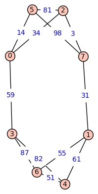
Dijkstra’s algorithms finds shortest paths in graphs with directed, weighted edges. In the following example of a symmetric (i.e. undirected) graph is, a shortest path from node 2 to node 4 would go via node 1 and node 7.
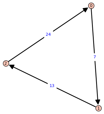
An example of a directed graph would be the following triangle, in which shortest pathes between nodes are unique.
One can implement Dijkstra’s algorithm via MPI: Every worker gets assigned a fixed set of nodes. In every iteration, each worker updates its unvisited neighbore to the current node. The minimal tentative distance among all nonvisited nodes can also be determined by a distributed computation.
Using MPI on Gantenbein
MPI on Gantenbein is organized as a module. Before using it run
module load mpi
Implementation
Implement the described algorithm as a program called dijkstra in C using MPI. The program should output the length of a shortest path in the graph from a given source to a given destination.
mpirun -n 1 dijkstra 2 4 example_graph
You can call an example program via
mpirun -n 1 /home/hpc2018/a5_example/dijkstra 1 17 /home/hpc2018/a5_grading/test_data/graph_de1_ne3_we2
Graph input file
Your program should read the graph from a given file with lines of the form
i1 i2 w
where i1 and i2 are indices of vertices connected by an edge of weight w. The first two columns are the lable of a vertices, a positive integer, and the third one is a weight, an integer greater than 0. The above graph would, for example, yield
6 4 51
5 2 81
0 5 14
5 0 14
6 1 55
2 7 3
7 5 98
3 4 82
3 0 59
6 3 87
1 4 61
5 7 98
7 2 3
2 5 81
1 6 55
4 3 82
0 2 34
0 3 59
3 6 87
4 1 61
1 7 31
4 6 51
2 0 34
7 1 31
Note that the this graph has undirected edges, so that the table of weights is symmetric.
Examples of Graphs
You can find a list of test graphs at
/home/hpc2018/a5_grading/test_data
There is also a python script, that you can use to generate test cases for you convenience.
Test script
You can check your submission with the script
/home/hpc2018/a5_grading/check_submission.py PATH_TO_SUMISSION.tar.gz
Performance goals
For the files that can be found at
/home/hpc2018/a5_grading/test_data
| Degree | 10 | 100 | 100 | 100 | 1000 |
| Number of vertices | 1000 | 10000 | 10000 | 100000 | 100000 |
| Maximal weight | 100 | 100 | 100 | 100 | 1000 |
| File name | graph_de1_ne3_we2 | graph_de2_ne4_we2 | graph_de2_ne4_we2 | graph_de2_ne5_we2 | graph_de3_ne5_we3 |
| Number of nodes | 1 | 1 | 4 | 10 | 20 |
| Start point | 9 | 17 | 17 | 107 | 4 |
| End point | 82 | 40 | 18 | 0 | 5 |
| Time in seconds | 1.2 | 6.8 | 3.1 | 98 | 256 |