A
streamline problem
In this assignment you will visualize some vector data in 3D. Such data
often comes from CFD (Computational Fluid Dynamics) or CEM
(Computational Electromagnetics), but since this is not a course in
those subjects, you will create some data in an easier way. We have a
system of ODE (Ordinary Differential Equations):
(eq1)
u'(t) = f(t, u, v)
v'(t) = g(t, u, v)
f and g are given functions and we are looking for u and v.
Such a system usually has infinitely many solutions (since we do not
have any initial conditions). If we apply some initial conditions, u(0)
and v(0) have prescribed values, we usually get a unique solution. The
solutions are usually plotted as 2D-curves, (t, u(t)) and (t, v(t)).
Another common way is to plot (u(t), v(t)) in a 2D-plot (the phase
plane). Less common is to plot (t, u(t), v(t)) as a 3D-curve but that
is roughly what you should do in this assignment, for different sets of
initial values.
Here is the problem. We want to get a feeling for what all the solutions
of (eq1) look like (where t, u and v are bounded). You have probably
done that for one equation, u'
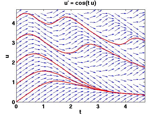
= f(t, u), so let us first look at such an example. Take u' = cos(t u).
We start by creating a mesh, in the
(t, u) plane. In every point in the mesh we draw an arrow having the
same direction as the solution, u, going through that curve. Here
is a typical plot. The vector field is in blue and I have used ode45 to compute some solutions
(with given initial conditions) in red.
Note that we can draw the arrows without having to solve the
differential equation. The derivative, u'(t), i.e. the direction of the
arrow in (t, u), is given by cos(t u), since u'(t) = cos(t u). Given
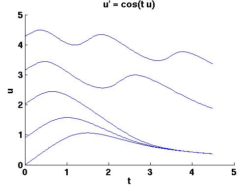
the data for the arrows we can use Matlab's streamline routine to
approximate some solutions like this:
Now to the problem.
 We have the ODE, two equations
this time (so the above plots will be generalized to three dimensions):
We have the ODE, two equations
this time (so the above plots will be generalized to three dimensions):
u'
= a u + b v + 0.2 cos t
v' = -b u + a v + 0.5 sin t, a =
-0.23, b = -2
Use Matlab to produce suitable data. Check your data using Matlab's streamline,
streamtube and quiver3 commands (so I want to
see Matlab plots as well).
Write an OpenDX-program where we can choose (choose an interactor, such
as Selector or Integer and combine with Route) to see one of
glyphs,
streamline, tubes and ribbons (so four choices) in three
dimensions.
A reasonable region is t in [0, 10], u and v in [-5, 5] or so.
Hint: you can use the
Grid-module to produce starting points for the streamlines. It may not
be crystal clear how to use it so here is an example. Suppose you have
numbered your variables so that t comes first and then u and v. The
following settings in Grid will produce all possible combinations of
points [0,
u, v] where u = linspace(-2, 2, 4), v = linspace(-3, 3, 8) to use
Matlab notation. This is an example, do not use these settings! I used
AutoGlyph to check the positions, that is the reason for Destination
being AutoGlyph. Not so in the lab.