Instructions
Your solution to assignments should be packaged as a tar.gz archive named by your lower case last name, and send it to me on the due day at the lastest.
Assignments may consist of several tasks, each of which should be implemented using the indicated programming language. Each task should be implemented in a separate folder, and the main file for each task should follow the given naming convention. If your solution to an exercise has more then one file, then include a make file that builds the program.
In addition to the source code, you have to write a report in (pandoc compatible) markdown that explains your solution and answers all questions posed in context of the task. This report should be called “report.markdown” and be placed in the root folder of your solution archive. If you include any addition material (like pictures and graphs) in your report, then this should be contained in the folder material. I will compile the report using pandoc, so make sure to comply with its syntax.
For example, in assignment 1, you have subtasks whose main files ought to be called “benchmark”, “profiling”, etc. A viable hand in by myself would thus be a file “westerholt.tar.gz” which contains a the file “report.markdown” and folders named “material”, “benchmark”, “profiling”, etc. The material contains an image “profile_graph.png”, which is linked to from the report. The benchmark folder contains a “main.c” and several other C-files “addition.c”, “sin.c”, etc. Beyond that it contains a makefile, which when invoked builds the program main.
Overview
There are five assignments in total. The first due date is rather late in after the start to provide sufficient time to get acquainted with HPC. Do not underestimate the time it takes to solve an assignment. Notice that there are no lab sessions (and no lectures) during the week of April 25 to 29.
| Name | Due Date | Description |
|---|---|---|
| optimization | April 29, 2016 | Performance measurement, diagnosis, and basic optimization. |
| threads | May 12, 2016 | POSIX threads. |
| openmp | May 19, 2016 | OpenMP, a compiler parallelization framework. |
| mpi | May 26, 2016 | Message passing interface for distributed computing. |
| opencl | May 26, 2016 | Framework for heterogeneous computing environment (GPU, FMPG, etc.). |
Assignment 1: Optimization
→ Back to the overview of assignments
The goal of the first assignment is to practice how to benchmark and profile code, and to inspect what major aspects contribute to performance. your code and the report as instructed.
Benchmarking
Write a C program, called benchmark, that approximates the time to perform a single
- addition,
- addition-multiplication,
- division,
- sin, and
- exp
provided that one executes many of them in a row. Carry out this measurement for float, double, and the first three also for long int. For example, you would measure how long a single addition of two doubles takes when executing 100,000 of them.
In your report, summarize the time you have measured (of what), the number of operators per second, and the compiler flags and the architecture that you have performed the test with. Comment on your result, and in particular, cross check them from a theoretical point of view.
Locality
Write a C or C++ program, called locality, that
- creates a matrix of doubles of size 1000 x 1000,
- stores them in a matrix in row first order,
- computes the row and the column sums.
Use naive implementations of row and column sums:
void
row_sums(
  double * sums,
  const double ** matrix,
  size_t nrs,
  size_t ncs
)
{
  for ( size_t ix=0; ix < nrs; ++ix ) {
    double sum = 0;
    for ( size_t jx=0; jx < ncs; ++jx )
      sum += matrix[ix][jx];
    sums[ix] = sum;
  }
}

void
col_sums(
  double * sums,
  const double ** matrix,
  size_t nrs,
  size_t ncs
  )
{
  for ( size_t jx=0; jx < ncs; ++jx ) {
    double sum = 0;
    for ( size_t ix=0; ix < nrs; ++ix )
      sum += matrix[ix][jx];
    sums[jx] = sum;
  }
}
Benchmark them according to the above scheme (executing 50 times will suffice). Compare timings and reimplement the slower summation in a more effective way. In addition, compile your program with and without full optimization. Summarize your benchmark results in a short table.
Indirect addressing
Indirect addressing is frequently used for sparse matrix and vector operators. Write a C or C++ program that increments a vector y by a multiple of a vector x. Both vectors will have same length 1,000,000 and the index vector (as opposed to real world applications) has also that length.
Implement, as a program called indirect_addressing, code
n = 1000000; m = 1000;
for (kx=0; kx < n; ++kx) {
  jx = p[kx];
  y[jx] += a * x[jx];
}
and benchmark it with some vectors x and y, and scalar a, and with p generated by either
ix = 0;
for (jx=0; jx < m; ++jx)
  for (kx=0; kx < m; ++kx)
    p[jx + m*kx] = ix++;
or
for (ix=0; ix < n; ++ix)
  p[ix] = ix;
Also implement and benchmark the same operation without indirect addressing, i.e. by accessing x and y directly.
Use full optimization in all cases. Compare the two timings, and explain the difference.
Inlining
Implement a function
void
mul_cpx( double * a_re, double * a_im, double * b_re, double * b_im, double * c_re, double * c_im)
that computes the product of two complex numbers b and c, and stores it in a. Store it as a separate file, and write a program inlining, that generates vectors a, b, and c of length 30,000, generates entries for b and c, and then multiplies their entries, saving them to a. Benchmark this.
Inline the code of for multiplication, by hand, in the loop over a, b, and c. Benchmark once more, and compare the result. Reason about the difference.
LAPack
The Cholesky decomposition of a positive definite, symmetric matrix A is C C^t for a lower trigonal matrix C. A naive inplace implementation of the Cholesky decomposition could be
double
dot(
  double * x,
  double * y,
  size_t jx
)
{
  double sum = 0;
  for (size_t ix = 0; ix < jx; ++ix)
    sum += x[ix] * y[ix];
  return sum;
}

for (size_t jx = 0; jx < nrs; ++jx) {
  double row_sum = 0;
  for ( size_t ix = 0; ix < jx; ++ix )
    row_sum += A[jx][ix] * A[jx][ix];
  A[jx][jx] = sqrt(A[jx][jx] - row_sum);

  for (size_t ix = jx+1; ix < nrs; ++ix)
    A[ix][jx] = ( A[ix][jx] - dot(A[ix], A[jx], jx) ) / A[jx][jx];
}
Implement the above in algorithm in a program called lapack, and benchmark it for a matrices of sizes 50, 100, up to , 1500. Compute the Cholesky decomposition by the GNU Scientific Library, and by PLASMA using 3 cores (To install PLASMA locally, you can use the PLASMA installer). Benchmark them, too, plot all obtained timings, and compare.
Positive definite, symmetric matrices
Given any invertible matrix B, then A = B B^t is positive definite and symmetric. In particular, you can start with, say, an upper trigonal matrix B whose diagonal entries are nonzero.
Profiling
Using the tools gprof and gcov to inspect your own implementation of the Cholesky factorization for matrix size 1000. Identify the parts of your implementation that are most time consuming. Also identify those parts that are most frequently run.
Assignment 2: Threads
→ Back to the overview of assignments
We will use Newton’s method to practice programming with POSIX threads. Give a function f, say f(x) = x^3 - 1, Newton’s method iteratively strives to find a root of f. Starting with a value x_0, one sets x_{k+1} = x_k - f(f_x) / f’(x_k). Convergence of this is unclear, and even if it does converge, it is unclear what root of f is approached.
Here is an example run of Newton’s method for three different (complex) values of x_0.
| real value | complex value | complex conjucate of previous one | |
|---|---|---|---|
| x_0 | 4.00000000000000 | -3.00000000000000 + 1.00000000000000i | -3.00000000000000 - 1.00000000000000i |
| x_1 | 2.68750000000000 | -1.97333333333333 + 0.686666666666667i | -1.97333333333333 - 0.686666666666667i |
| x_2 | 1.83781773931855 | -1.25569408339907 + 0.505177535283118i | -1.25569408339907 - 0.505177535283118i |
| x_3 | 1.32390198935733 | -0.705870398114610 + 0.462793270024375i | -0.705870398114610 - 0.462793270024375i |
| x_4 | 1.07278230395299 | -0.284016534261040 + 0.737606186335893i | -0.284016534261040 - 0.737606186335893i |
| x_5 | 1.00482620484690 | -0.585120941952759 + 0.849582155034797i | -0.585120941952759 - 0.849582155034797i |
| x_6 | 1.00002314326798 | -0.501764864834321 + 0.859038339628915i | -0.501764864834321 - 0.859038339628915i |
| x_7 | 1.00000000053559 | -0.499955299939949 + 0.866052541624328i | -0.499955299939949 - 0.866052541624328i |
One can experimentally find which points on the complex plane converge to which root. Below there are two pictures: In the left one every pixel is colored in such a way that its color corresponds to the root which it converges to. In the right hand side every, every pixel is color in such a way that its color corresponds to the number of iterations which are necessary to get close to a root of f. Note that this computation can be carried out for each pixel in parallel. There is no interdependence of the iterations.


Implement in C or C++ using POSIX threads a program called newton_pngs that computes similar pictures for a given functions f(x) = x^n - 1 for complex numbers with real and imaginary part between -2 and +2. The program should write the results as png files of width and height 1000 to the current working directory. The files should be named newton_attractors_xn.png and newton_convergence_xn.png where n is replaced by the exponent of x that is used.
Your program should use a fixed number of threads determined by a runtime argument:
./newton_pngs -t5 7should use 5 threads and compute pictures for x^7 - 1. The implementation should compute the pictures row by row. A load balancer should assign to each idle thread the next row to compute. One one thread should access the png data structure, while all others are exclusively computing Newton iterations.
In your report, explain your conception of your load balancer.
PNG files
There is a convenient C++ wrapper png++ for libpng, with documentation available. Install and compile png++ from [download.savannah.gnu.org/releases/pngpp].
Assignment 3: OpenMP
→ Back to the overview of assignments
In this assignment, we count in parallel distances between points in 3-dimensional space. On possibility to think of this, is as cells whose coordinates were obtained by diagnostics, and which require further processing.
Implement a program in C or C++, called cell_distances, that uses OpenMP and that
- reads coordinates of cells from a text file “cells” in the current working directory,
- computes the distances between cells counting how often each distance rounded to 2 digits occurs, and
- outputs to stdout a list of distances that occurred.
Distances are symmetric, i.e. distance between two cells c_1 and c_2 and the distance in reverse direction c_2 to c_1 should be counted once.
You may not first compute all distances and then process them: In real world applications this exceeds by fare the capacities of computers.
Benchmark your implementation with the example file using 1,2,3, and 4 threads, and discuss the timings.
Example
The list of positions is given as a file of the form
0.843 0.598 0.406
0.175 0.429 0.530
0.053 0.449 -0.792
-0.940 0.612 -0.946
0.523 0.99 0.831
-0.704 0.672 0.646
0.260 0.617 -0.163
-0.132 -0.838 -0.013
0.626 0.824 -0.882
0.645 0.412 -0.009
A valid output is
0.46 1
0.50 1
0.66 1
0.68 1
0.69 1
0.70 1
0.72 2
0.73 1
0.81 1
0.83 1
0.92 1
0.97 1
0.98 1
1.02 1
1.03 1
1.09 1
1.26 1
1.28 1
1.33 2
1.41 1
1.43 1
1.44 1
1.47 1
1.51 1
1.52 2
1.53 1
1.57 1
1.58 1
1.61 1
1.64 1
1.72 1
1.74 1
1.77 1
1.79 1
1.85 1
1.86 1
1.90 1
2.02 1
2.03 1
2.12 1
2.24 1
2.33 1
Assignment 4: MPI
→ Back to the overview of assignments
There are two subtasks for this assignment, the first of which is a basic exercise to get acquainted with MPI.
Running MPI on student servers
You can run an mpi program main using two processes by
mpiexec -n 2 ./mainThe IT-infrastructure for this course is centered around Ozzy. In this section, let us assume that we worked with five remote machines available to run MPI process: remote1.studat.chalmers.se through remote5.studat.chalmers.se. To run MPI on them you could, for example, create a host file, call it hostfile,
remote1.studat.chalmers.se
remote2.studat.chalmers.se:2
remote3.studat.chalmers.se:3
remote4.studat.chalmers.se
remote5.studat.chalmers.se:3
and then invoke MPI by
mpiexec -f hostfile ./mainOne example
The next code, would let each process print its rank and the host it is executed on.
Using the host file
remote1.studat.chalmers.se:2
remote3.studat.chalmers.se:2
remote5.studat.chalmers.se:3
we might receive the following output
  mpiexec -f hostfile ./main
0 remote1.studat.chalmers.se
1 remote5.studat.chalmers.se
4 remote1.studat.chalmers.se
3 remote3.studat.chalmers.se
2 remote3.studat.chalmers.se
5 remote5.studat.chalmers.se
The order may vary depending on your situation.
#include <stdio.h>
#include <unistd.h>
#include "mpi.h"

int
main(
  int argc,
  char **argv
  )
{
  int mpi_rank;
  size_t len = 50;
  char host_name[len];

  MPI_Init(&argc, &argv);
  MPI_Comm_rank(MPI_COMM_WORLD, &mpi_rank);

  gethostname(host_name, len);
  printf("%2d %s\n", mpi_rank, host_name);

  MPI_Finalize();
  return 0;
}
Debugging
Since MPI buffers output, it might be necessary to flush the stdout buffer, when debugging with print statements. In C and C++ this is done by
fflush(stdout);
cout.flush();
Note that in C++ the error stream cerr is flushed automatically after each write.
Enumerating MPI workers
Implement a program, called mpi_worker_count, in C or C++ consisting of one MPI master and several MPI workers with the following behavior:
- the master sends to the first work the integer 0,
- every works increases the integer it receives by 1 and forwards this to the next worker (if it is not the last one),
- the last worker forwards the integer to the master, that prints it.
The result, obviously, is the number of workers.
Dijkstra’s shortest path algorithm
Dijkstra’s algorithms finds shortest paths in graphs with weighted edges. In the next example of such a graph is, a shortest path from node 2 to 4 would go via 1 and 7.
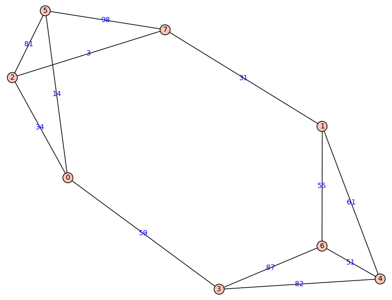
One can implement Dijkstra’s algorithm via MPI: Every worker gets assigned a fixed set of nodes. In every iteration, each worker updates its unvisited neighbors to the current node. The minimal weights are reduced, and the worker that is assigned this node broadcasts its index.
Implement the described algorithm as a program called dijkstra in C or C++ using MPI. Run it on random d-regular graphs (i.e. every node has d edges) with n nodes for (d;n) equal to (100;2,000), (100;10,000) and (1000;10,000) with 2, 5, and 10 workers on a suitable number of hosts. Benchmark these, summarize the timings in a short table, and reason about them.
Examples of Graphs
You can find files with examples of graph of parameters (5,100), (100,2000), (100,10000), and (1000,10000). Graphs described by the data in the files have vertices enumerated starting at 0. The files contain lines of the form
i1 i2 wwhere i1 and i2 are indices of vertices connected by an edge of weight w.
Assignment 5: OpenCL
→ Back to the overview of assignments
A simple model for heat diffiusion in 2-dimensional space, splits it up into n_x times n_x small boxes. In each time step, the temperature h(i,j) of a box with coodinates i and j is updated as
h(i,j) + c * ( (h(i-1,j) + h(i+1,j) + h(i,j-1) + h(i,j+1))/4 - h(i,j) )
where c is a diffision constant. We consider the case of bounded region of box shape whose boundary has constant temperature 0.
Implement in C using the GPU via OpenCL a program heat_diffusion that
- initializes an array of given size to 0 except for the middle point whose value should be 1,000,000,
- executes a given number of steps of heat diffusion with given diffusion constant, and
- outputs the average absolute difference of each temperature to the average of all temperatures.
For example,
heat_diffusion 1000 2000 0.02 20should compute 20 steps of heat diffusion on a 1000 times 2000 boxes with diffusion rate 0.02.
Implement the same algorithm using CPU arithmetic, and benchmark both.
Example
As an example, we consider the case of 3 times 3 boxes with diffusion constant 1/30. Their initial heat values written in a talbe are
| 0 | 0 | 0 |
| 0 | 1,000,000 | 0 |
| 0 | 0 | 0 |
Then the next two iterations are
| 0.000 | 8333. | 0.000 |
| 8333. | 9.667e2 | 8333. |
| 0.000 | 8333. | 0.000 |
and
| 138.9 | 1611e1 | 138.9 |
| 1611e1 | 9347e2 | 1611e1 |
| 138.9 | 1611e1 | 138.9 |
In particular, the average temperature is 111080. (as opposed to the original average 111111.), and the absolute difference of each temperature and the average is
| 1109e2 | 9497e1 | 1109e2 |
| 9497e1 | 8236e2 | 9497e1 |
| 1109e2 | 9497e1 | 1109e2 |
The average of this is 183031.55. After five further iterations this will decrease to 151816.97.